Visualization

tralda.visualization draws Tree objects (see Trees) as publication-ready figures or interactive plots. It ships two independent backends — matplotlib for static figures and Plotly for interactive HTML — behind a shared layout and styling API, so the same tree and styling logic can be rendered with either one.

This page is a quick start. For the full styling and layout API see Layout & Styling; for two complete worked examples (a real phylogeny and a simulated dataset) see Examples.

Installation

The renderers are optional extras and are not installed by default:

pip install tralda[matplotlib]   # static figures
pip install tralda[plotly]       # interactive HTML / static image export
pip install tralda[viz]          # both

Importing tralda.visualization itself never requires either package — the renderer classes are imported lazily on first use, so you only need the backend(s) you actually use.

The one-liner: plot_tree

For the common case, plot_tree lays out and renders a tree in a single call:

from tralda.datastructures import Tree
from tralda.visualization import plot_tree

T = Tree.parse_newick(
    "((((Human:6,Chimpanzee:6)HC:2,Gorilla:8)HCG:9,Orangutan:17)Hominidae:3,"
    "(Gibbon:17,Siamang:17)Hylobatidae:3)Hominoidea;"
)

fig, ax = plot_tree(T)  # set show_internal_labels=True to display internal node labels
fig.savefig("tree.png")

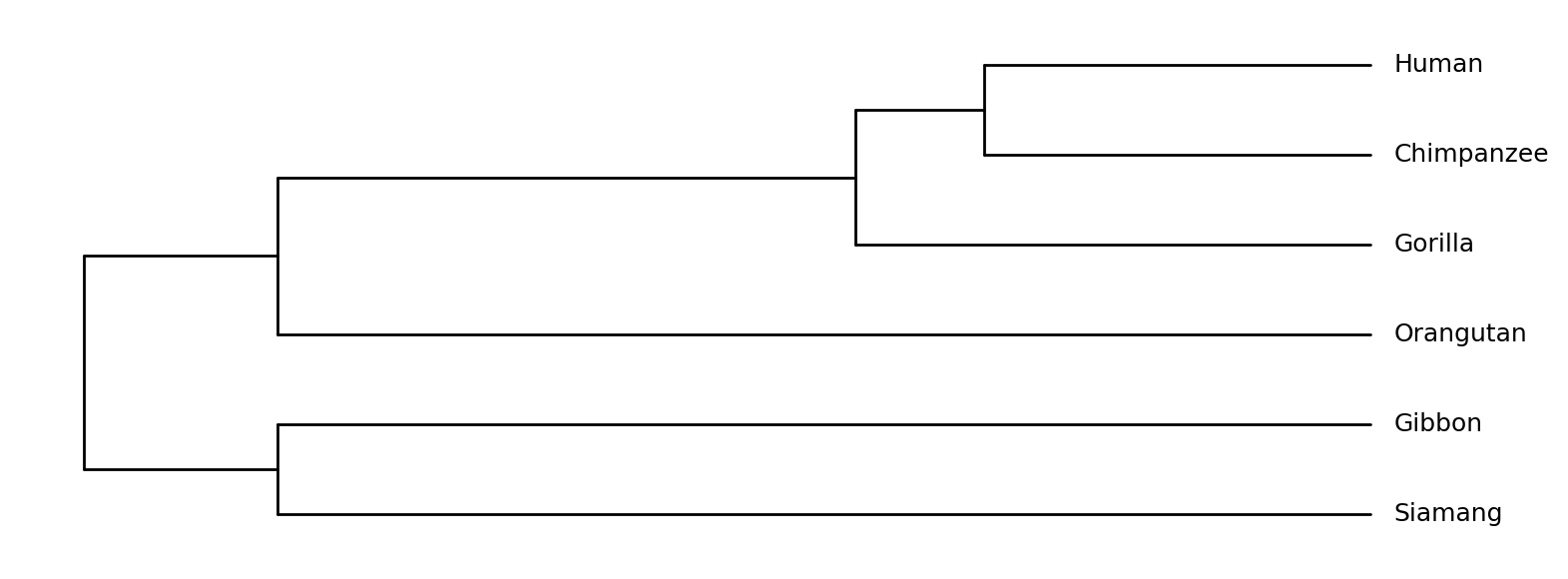
(Branch lengths above are illustrative divergence times, not scientifically exact.)

Pass backend="plotly" to get an interactive figure instead, and path=... / show=True to save and/or immediately display the result:

plot_tree(T, backend="plotly", path="tree.html", show=True)

Architecture

Three concerns are deliberately kept separate, which is what makes it possible to reuse the same tree geometry across renderers, or the same styling across layouts:

Class	Responsibility
TreeLayout	Computes (x, y) positions for every node once, given a layout mode and edge-length mode.
TreeStyle / NodeStyle	Resolves colors, symbols, and label styling per node.
MatplotlibRenderer / PlotlyRenderer	Consume a TreeLayout (and optionally a TreeStyle) and produce a figure.

plot_tree simply wires these three together. For anything beyond the default look — a different layout mode, custom colors, drawing onto an existing matplotlib Axes, or reusing one layout with several styles — construct them directly:

from tralda.visualization.layout import TreeLayout
from tralda.visualization.matplotlib_renderer import MatplotlibRenderer
from tralda.visualization.style import NodeStyle, TreeStyle

layout = TreeLayout(T, edge_length_mode="attr", layout_mode="horizontal")
style = TreeStyle(leaf_symbol="circle", default=NodeStyle(symbol_color="steelblue"))
fig, ax = MatplotlibRenderer(layout, tree_style=style, show_internal_labels=True).render()

Matplotlib vs. Plotly

Both renderers accept a TreeLayout and a TreeStyle and produce visually equivalent output; which one to reach for mostly depends on what you need afterwards:

• MatplotlibRenderer — returns (fig, ax). Use it for static output (.png, .pdf, .svg), for embedding in a larger matplotlib figure via the ax constructor argument, or when you need full control over a publication-quality plot.
• PlotlyRenderer — returns a plotly.graph_objects.Figure. Use it for interactive exploration (zoom, pan, hover tooltips showing node attributes via hover_attrs) and for self-contained HTML output (fig.write_html(...)). Static image export (fig.write_image(...)) requires the kaleido package (included in the plotly extra).

from tralda.visualization.plotly_renderer import PlotlyRenderer

renderer = PlotlyRenderer(layout, tree_style=style, hover_attrs=["dist"])
fig = renderer.render()
fig.write_html("tree.html")

Next: Layout & Styling for the full set of layout modes, edge-length modes, and styling mechanisms, or jump straight to Examples for two end-to-end examples with real and simulated data.